1  Module 1 — Data Preparation & Standardization

1.1 Learning Outcomes

By the end of this module learners will be able to:

• Explain the difference between normalization and standardization and when to use each.
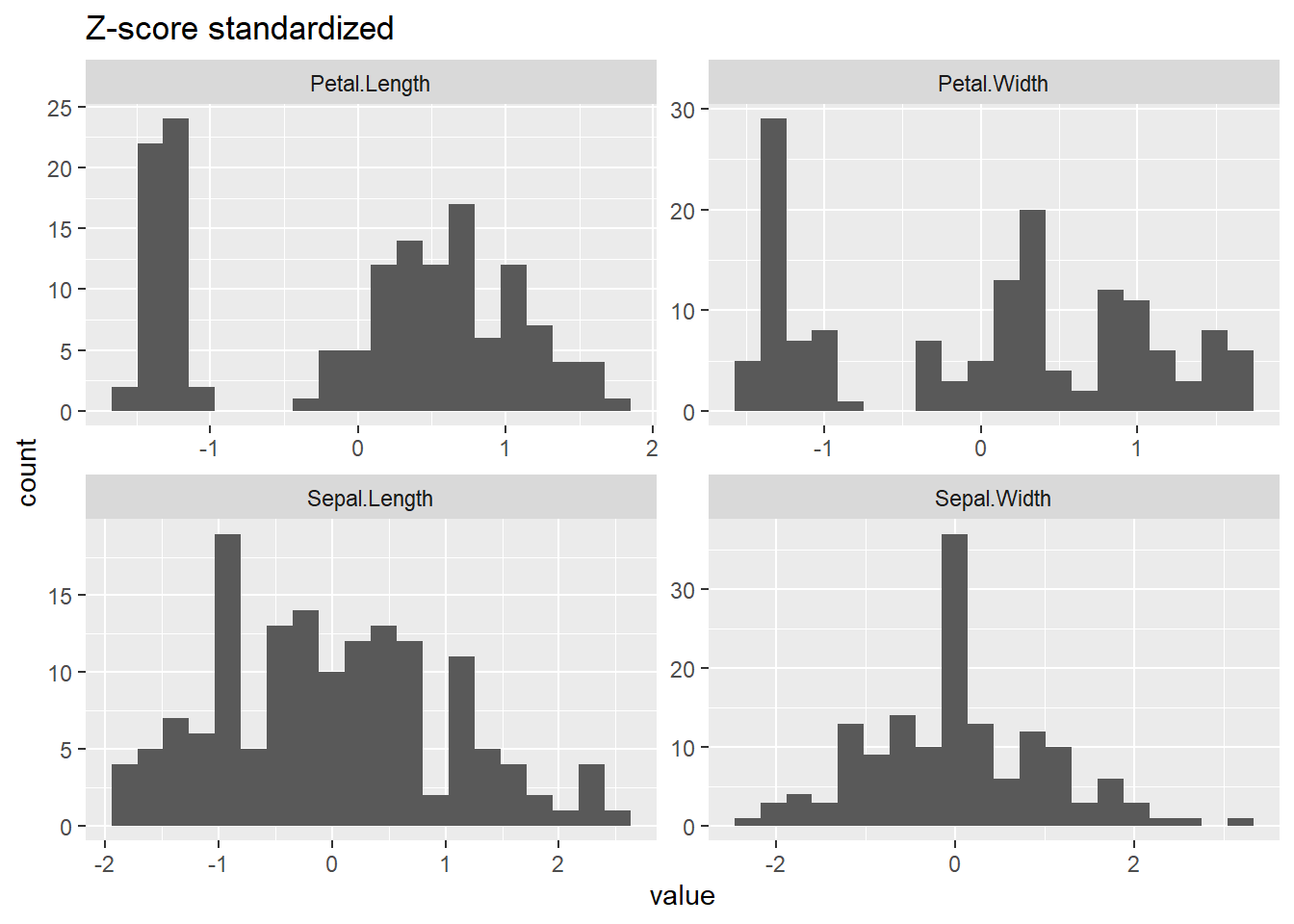
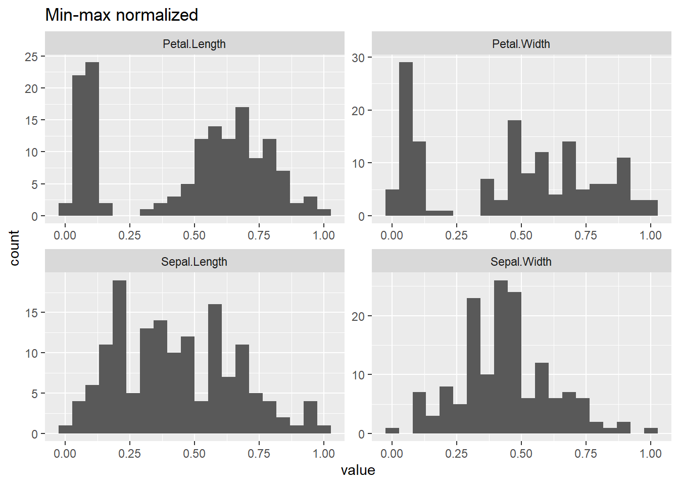
• Apply scaling methods in R (scale(), caret::preProcess) and create min-max and robust scaling.
• Detect and treat missing values and common outliers.
• Prepare data for PCA and clustering (center, scale, and check assumptions).
• Write small self-check tests to verify preprocessing steps.

---

1.2 1. Why preprocessing matters

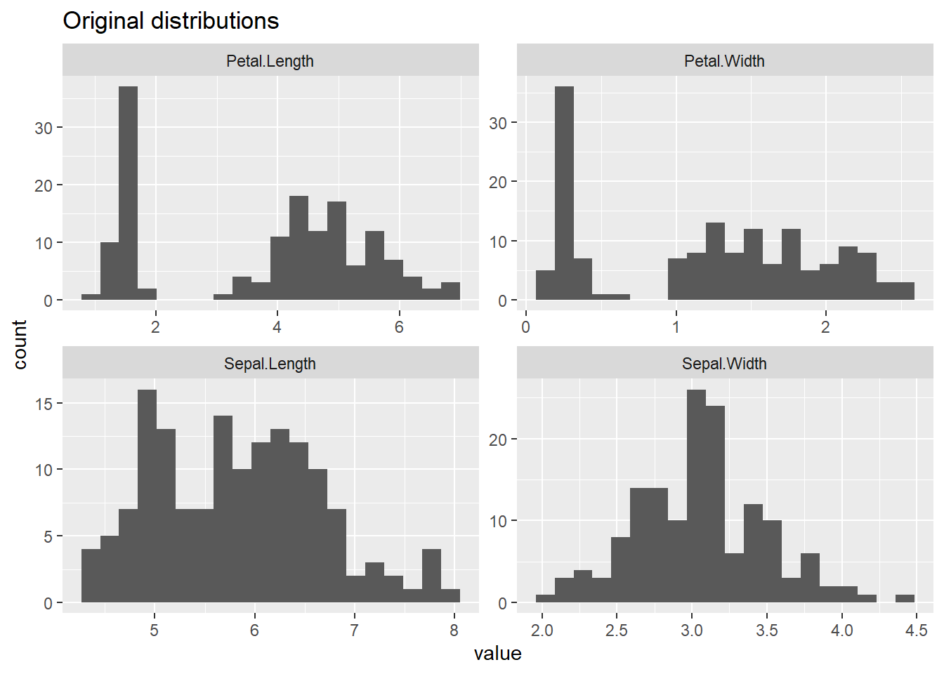
Many algorithms (like K-means, PCA, distance-based methods) assume features are on comparable scales. Preprocessing ensures that units and magnitudes don’t distort the analysis.

---

1.3 2. Data types and missing values

1.3.1 Inspecting structure

str(iris)

'data.frame':   150 obs. of  5 variables:
 $ Sepal.Length: num  5.1 4.9 4.7 4.6 5 5.4 4.6 5 4.4 4.9 ...
 $ Sepal.Width : num  3.5 3 3.2 3.1 3.6 3.9 3.4 3.4 2.9 3.1 ...
 $ Petal.Length: num  1.4 1.4 1.3 1.5 1.4 1.7 1.4 1.5 1.4 1.5 ...
 $ Petal.Width : num  0.2 0.2 0.2 0.2 0.2 0.4 0.3 0.2 0.2 0.1 ...
 $ Species     : Factor w/ 3 levels "setosa","versicolor",..: 1 1 1 1 1 1 1 1 1 1 ...

summary(iris)

  Sepal.Length    Sepal.Width     Petal.Length    Petal.Width   
 Min.   :4.300   Min.   :2.000   Min.   :1.000   Min.   :0.100  
 1st Qu.:5.100   1st Qu.:2.800   1st Qu.:1.600   1st Qu.:0.300  
 Median :5.800   Median :3.000   Median :4.350   Median :1.300  
 Mean   :5.843   Mean   :3.057   Mean   :3.758   Mean   :1.199  
 3rd Qu.:6.400   3rd Qu.:3.300   3rd Qu.:5.100   3rd Qu.:1.800  
 Max.   :7.900   Max.   :4.400   Max.   :6.900   Max.   :2.500  
       Species  
 setosa    :50  
 versicolor:50  
 virginica :50  
                
                
                

1.3.2 Handling missing values

set.seed(42)
iris_miss <- iris 
idx <- sample(seq_len(nrow(iris_miss)), size = floor(0.05 * nrow(iris_miss) ))
iris_miss$Sepal.Length[idx] <- NA
sum(is.na(iris_miss$Sepal.Length))

[1] 7

iris_drop <- na.omit(iris_miss)
iris_meanimp <- iris_miss
iris_meanimp$Sepal.Length[is.na(iris_meanimp$Sepal.Length)] <- mean(iris_meanimp$Sepal.Length, na.rm = TRUE)

#iris_miss %>% mutate(Sepal.Length = tidyr::replace_na(Sepal.Length,mean(iris_miss$Sepal.Length,na.rm = T))) %>% head()

# preProc <- preProcess(iris_miss[,1:4], method = c("knnImpute"))
# iris_knnimp <- predict(preProc, iris_miss[,1:4])

Discussion: When to delete (MCAR small portion) vs impute (MAR, domain knowledge). Mention advanced methods (MICE, missForest).

---

1.4 3. Normalization vs Standardization

1.4.1 Concepts

• scaling: involves dividing each value by the standard deviation.
• Centering: Centering subtracts the mean from each value.
• Normalization: Rescales to [0,1]. Useful for algorithms requiring bounded inputs.
• Standardization: Centers and scales to mean 0, SD 1. Ideal for PCA, K-means.
• Box-Cox Transform: Reduces skewness in data to make it more Gaussian-like.

1.4.2 Examples

num_iris <- iris %>% select_if(is.numeric)
z_iris <- scale(num_iris)
apply(z_iris, 2, function(x) c(mean = mean(x), sd = sd(x)))

      Sepal.Length  Sepal.Width  Petal.Length   Petal.Width
mean -4.484318e-16 2.034094e-16 -2.895326e-17 -3.663049e-17
sd    1.000000e+00 1.000000e+00  1.000000e+00  1.000000e+00

minmax <- function(x) (x - min(x)) / (max(x) - min(x))
mm_iris <- as.data.frame(lapply(num_iris, minmax))
apply(mm_iris, 2, range)

     Sepal.Length Sepal.Width Petal.Length Petal.Width
[1,]            0           0            0           0
[2,]            1           1            1           1

robust_scale <- function(x) (x - median(x)) / IQR(x)
robust_iris <- as.data.frame(lapply(num_iris, robust_scale))

1.4.3 Visualization

iris_long <- num_iris %>% mutate(row = row_number()) %>% pivot_longer(-row, names_to = "feature", values_to = "value")

p1 <- ggplot(iris_long, aes(x = value)) + geom_histogram(bins = 20) + facet_wrap(~feature, scales = "free") + ggtitle("Original distributions")

z_long <- as.data.frame(z_iris) %>% mutate(row = row_number()) %>% pivot_longer(-row, names_to = "feature", values_to = "value")

p2 <- ggplot(z_long, aes(x = value)) + geom_histogram(bins = 20) + facet_wrap(~feature, scales = "free") + ggtitle("Z-score standardized")

mm_long <- mm_iris %>% mutate(row = row_number()) %>% pivot_longer(-row, names_to = "feature", values_to = "value")

p3 <- ggplot(mm_long, aes(x = value)) + geom_histogram(bins = 20) + facet_wrap(~feature, scales = "free") + ggtitle("Min-max normalized")

p1

p2

p3

---

1.5 4. Outlier detection and treatment

boxplot.stats(iris$Sepal.Length)$out

numeric(0)

# IQR rule
iqr_rule <- function(x) {
  q1 <- quantile(x, 0.25)
  q3 <- quantile(x, 0.75)
  iqr <- q3 - q1
  x < (q1 - 1.5 * iqr) |  x > (q3 + 1.5 * iqr)
}
out_flags <- iqr_rule(iris$Sepal.Length)
sum(out_flags)

[1] 0

winsorize <- function(x, probs = c(0.05, 0.95)) {
  qs <- quantile(x, probs = probs)
  pmin(pmax(x, qs[1]), qs[2])
}
winsorized <- winsorize(iris$Sepal.Length)
summary(winsorized)

   Min. 1st Qu.  Median    Mean 3rd Qu.    Max. 
  4.600   5.100   5.800   5.830   6.400   7.255 

Teaching point: Decide removal, transformation, or winsorization based on context.

---

1.6 5. Feature transformations

mt <- mtcars %>% mutate(mpg_log = log(mpg))
summary(mt$mpg_log)

   Min. 1st Qu.  Median    Mean 3rd Qu.    Max. 
  2.342   2.736   2.955   2.958   3.127   3.523 

bc_pp <- preProcess(mtcars, method = "BoxCox")
predict(bc_pp, mtcars)[1:3, 1:4]

                   mpg cyl     disp       hp
Mazda RX4     3.044522   6 8.797297 4.700480
Mazda RX4 Wag 3.044522   6 8.797297 4.700480
Datsun 710    3.126761   4 7.754245 4.532599

---

1.7 6. Principle Component Analysis

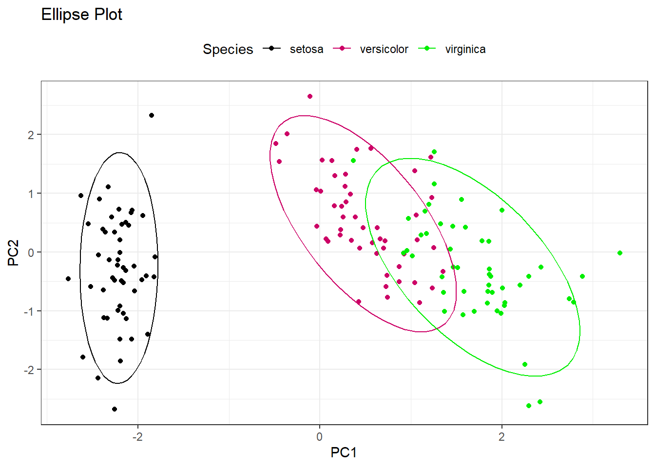
Principle Component Analysis is a transformation technique that focuses on dimensionaliity reduction. This entails transforming a dataset with a large number of variables into less variables that contain most of the information of the affected variables. The technique is split into 3 concepts as below

• Dimensionality Reduction where the large number of variables are condensed into smaller variables that are a representation of the large ones.
• Principal Components which are the new variables. These are a linear combination of the original variables and are ordered by the amount of the variance they capture.
• Variance: PCA assumes that the information is carried in the variance of the features. The higher the variation in a feature, the more information it carries.

1.7.1 Preparing for PCA

Checklist: - Handle missing values - Numeric only - Center and scale / standardization - Remove near-zero variance

pp_pipeline <- preProcess(iris[,1:4], method = c("center", "scale")) ## centering and scaling the data set
iris_scaled <- predict(pp_pipeline, iris[,1:4]) ## applying the behavior to the data set
pca_res <- prcomp(iris_scaled) ## getting the principle components
# summary(pca_res)
# plot(pca_res, type = "l", main = "Scree plot")

pca_dta <- pca_res$x %>%data.frame() 
pca_dta%>% head() %>%   flextable::flextable() %>% flextable::autofit()

PC1	PC2	PC3	PC4
-2.257141	-0.4784238	0.12727962	0.024087508
-2.074013	0.6718827	0.23382552	0.102662845
-2.356335	0.3407664	-0.04405390	0.028282305
-2.291707	0.5953999	-0.09098530	-0.065735340
-2.381863	-0.6446757	-0.01568565	-0.035802870
-2.068701	-1.4842053	-0.02687825	0.006586116

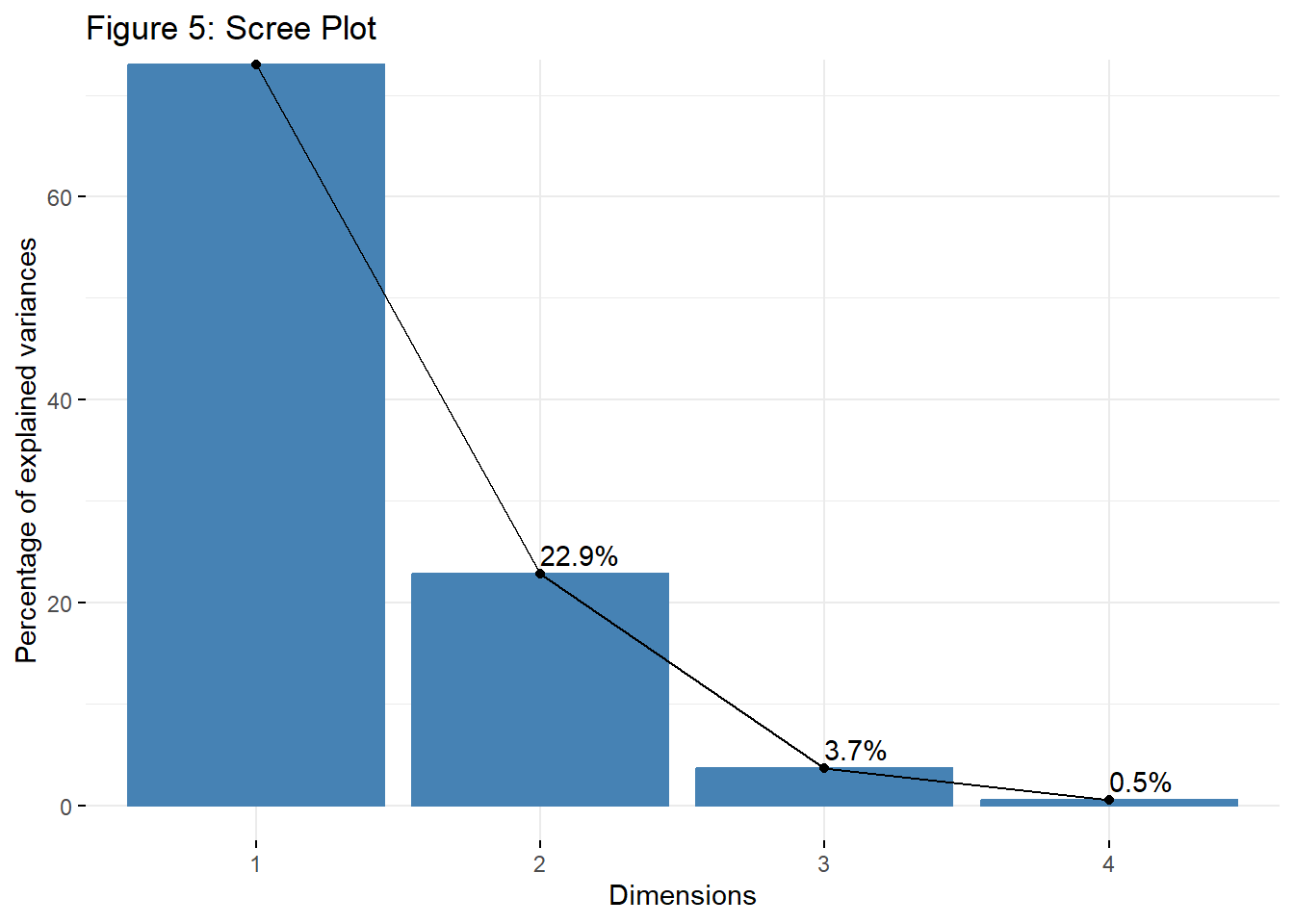
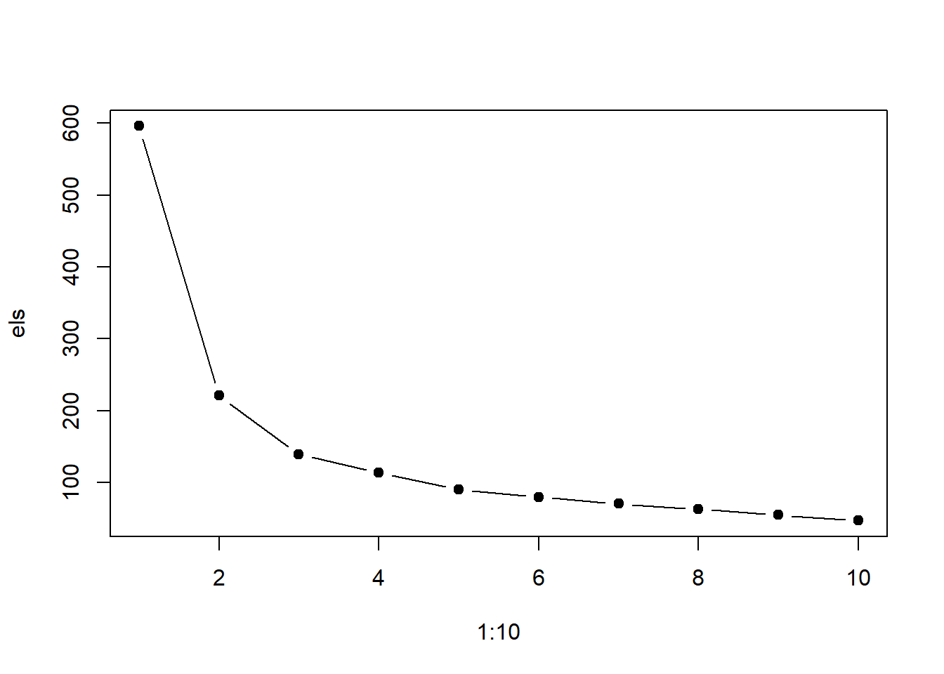
Visualizing the scree plot. This is used to visualize the eigenvalues or the proportion of variance explained by each principal component (PC).

library(factoextra)

Warning: package 'factoextra' was built under R version 4.3.3

Welcome! Want to learn more? See two factoextra-related books at https://goo.gl/ve3WBa

library(FactoMineR)

Warning: package 'FactoMineR' was built under R version 4.3.3

fviz_eig(pca_res, 
         addlabels = TRUE, 
         ylim = c(0, 70),
         main="Figure 5: Scree Plot")

Explaining the variance

pca_var <- pca_res$sdev^2
pca_var / sum(pca_var)

[1] 0.729624454 0.228507618 0.036689219 0.005178709

Comparing the PCA output and the current classifications

iris_pca <- pca_dta %>% bind_cols(iris %>% select(Species))

pca_dta$Species = iris$Species

# iris_pca %>% 
  ggplot(iris_pca,
       aes(x = PC1, 
       y = PC2, 
       color = Species)) +
       geom_point() +
       scale_color_manual(values=c("black", "#CC0066", "green2")) +
       stat_ellipse() + ggtitle("Ellipse Plot") +
       theme_bw()+
  theme(legend.position = "top")

---

1.8 7. Clustering

1.8.1 Learning Outcomes

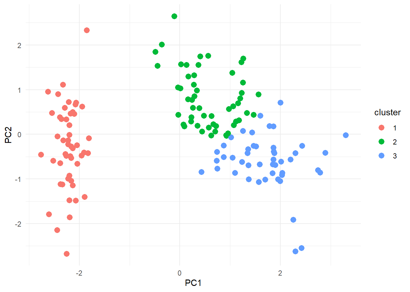
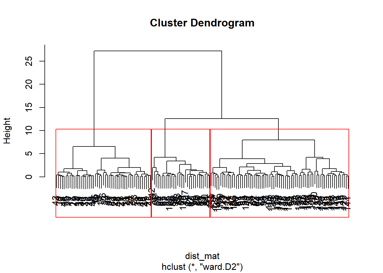
By the end of this module, learners will be able to: - Prepare data for clustering (scaling, distance measures, PCA-based preprocessing). - Perform K-Means, Hierarchical, and Density-Based clustering. - Evaluate clusters using Silhouette Width, Dunn Index, and internal metrics. - Interpret clusters visually using PCA and advanced plotting.

1.8.2 1. Data Preparation for Clustering

Before clustering, ensure variables are scaled correctly:

scaled_data <- scale(iris[,1:4])
head(scaled_data)

     Sepal.Length Sepal.Width Petal.Length Petal.Width
[1,]   -0.8976739  1.01560199    -1.335752   -1.311052
[2,]   -1.1392005 -0.13153881    -1.335752   -1.311052
[3,]   -1.3807271  0.32731751    -1.392399   -1.311052
[4,]   -1.5014904  0.09788935    -1.279104   -1.311052
[5,]   -1.0184372  1.24503015    -1.335752   -1.311052
[6,]   -0.5353840  1.93331463    -1.165809   -1.048667

Key concepts: - Distance-based algorithms require standardized input. - PCA helps reduce multicollinearity and compress correlated features.

---

1.8.3 2. K-Means Clustering (Deep Dive)

1.8.3.1 2.1 Running K-Means

set.seed(123)
kmeans_fit <- kmeans(scaled_data, centers = 3, nstart = 25)
kmeans_fit

K-means clustering with 3 clusters of sizes 50, 53, 47

Cluster means:
  Sepal.Length Sepal.Width Petal.Length Petal.Width
1  -1.01119138  0.85041372   -1.3006301  -1.2507035
2  -0.05005221 -0.88042696    0.3465767   0.2805873
3   1.13217737  0.08812645    0.9928284   1.0141287

Clustering vector:
  [1] 1 1 1 1 1 1 1 1 1 1 1 1 1 1 1 1 1 1 1 1 1 1 1 1 1 1 1 1 1 1 1 1 1 1 1 1 1
 [38] 1 1 1 1 1 1 1 1 1 1 1 1 1 3 3 3 2 2 2 3 2 2 2 2 2 2 2 2 3 2 2 2 2 3 2 2 2
 [75] 2 3 3 3 2 2 2 2 2 2 2 3 3 2 2 2 2 2 2 2 2 2 2 2 2 2 3 2 3 3 3 3 2 3 3 3 3
[112] 3 3 2 2 3 3 3 3 2 3 2 3 2 3 3 2 3 3 3 3 3 3 2 2 3 3 3 2 3 3 3 2 3 3 3 2 3
[149] 3 2

Within cluster sum of squares by cluster:
[1] 47.35062 44.08754 47.45019
 (between_SS / total_SS =  76.7 %)

Available components:

[1] "cluster"      "centers"      "totss"        "withinss"     "tot.withinss"
[6] "betweenss"    "size"         "iter"         "ifault"      

1.8.4 2.2 Visualizing K-Means Clusters

# 1. Scale data
scaled_data <- scale(iris[,1:4])

# 2. Run PCA
pca1 <- prcomp(scaled_data)
pca_scores <- as.data.frame(pca1$x[, 1:2])  # PC1 and PC2

# 3. Run K-means 
set.seed(123)
kmeans_fit <- kmeans(scaled_data, centers = 3, nstart = 25)

# 4. Build dataframe for plotting
cluster_df <- cbind(pca_scores, cluster = as.factor(kmeans_fit$cluster))

# 5. Plot
ggplot(cluster_df, aes(PC1, PC2, color = cluster)) +
  geom_point(size = 3) +
  theme_minimal()

1.8.4.1 2.3 Cluster Evaluation

Elbow Method:

els <- vector()
for (k in 1:10) {
  els[k] <- kmeans(scaled_data, centers = k, nstart = 20)$tot.withinss
}
plot(1:10, els, type = "b", pch = 19)

using another approach that considers the average silhouette

fviz_nbclust(scaled_data, kmeans, method = "silhouette")

Silhouette Score:

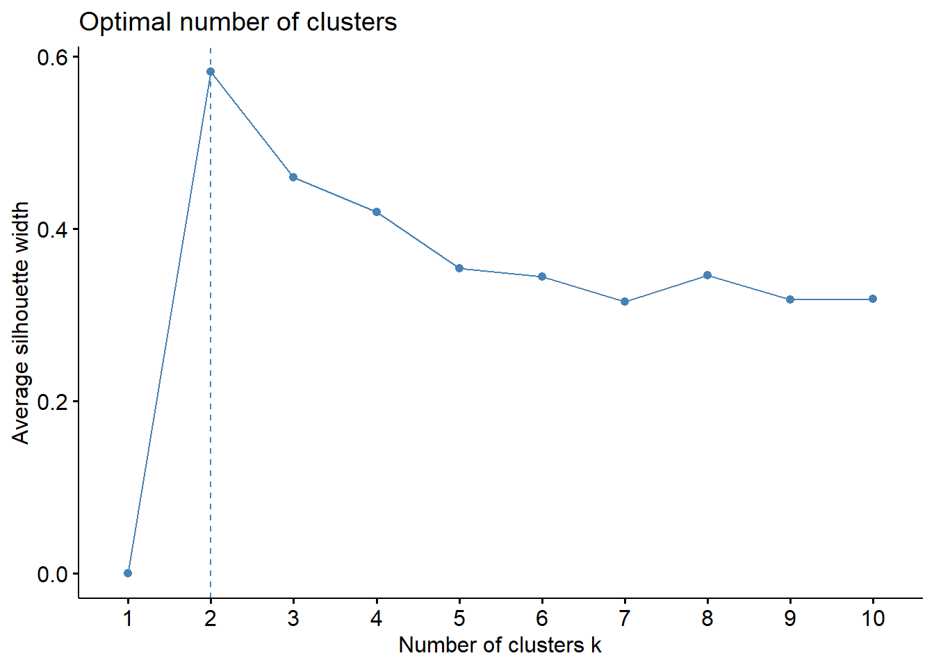
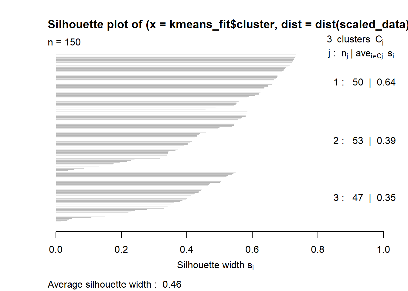
The Silhouette Score is used to evaluate the quality of clusters in a clustering algorithm. It measures how similar a sample is to its own cluster compared to other clusters. The score ranges from -1 to 1, where a higher score indicates better-defined clusters.A score close to 1 indicates that the sample is well-clustered, a score close to 0 indicates overlapping clusters, and a negative score indicates that the sample might be assigned to the wrong cluster.

library(cluster)
sil <- silhouette(kmeans_fit$cluster, dist(scaled_data))
plot(sil)

mean(sil[,3])

[1] 0.4599482

Interpretation: Scores close to 1 indicate well-separated clusters.

1.8.5 3. Hierarchical Clustering

dist_mat <- dist(scaled_data)
fit_hc <- hclust(dist_mat, method = "ward.D2")
plot(fit_hc)
rect.hclust(fit_hc, k = 3, border = "red")

Discussion: When to use hierarchical vs K-means.

### 4. DBSCAN (Density-Based Clustering)
  
# library(dbscan)
# set.seed(42)
# db <- dbscan(scaled_data, eps = 0.5, minPts = 5)
# plot(db, scaled_data)

Useful for non-spherical clusters; can detect noise.

---

## 7. Full pipeline example

# iris_num <- iris %>% select_if(is.numeric)
# nzv <- nearZeroVar(iris_num)
# iris_num2 <- iris_num[, -nzv]
# pp <- preProcess(iris_num2, method = c("scale"))
# iris_ready <- predict(pp, iris_num2)
# apply(iris_ready, 2, function(x) c(mean = mean(x), sd = sd(x)))

---

1.9 8. Exercises and Self-tests

Exercise 1: Write zscore_df() to z-score numeric columns.

Exercise 2: Write minmax_df() to normalize numeric columns.

Exercise 3: Write iqr_outliers() that returns indices of outliers.

zscore_df <- function(df){
  num <- df %>% select_if(is.numeric)
  as.data.frame(scale(num))
}
z_mtcars <- zscore_df(mtcars)
means <- sapply(z_mtcars, mean)
sds <- sapply(z_mtcars, sd)
stopifnot(all(abs(means) < 1e-8))
stopifnot(all(abs(sds - 1) < 1e-8))

minmax_df <- function(df){
  num <- df %>% select_if(is.numeric)
  as.data.frame(lapply(num, function(x) (x - min(x)) / (max(x) - min(x))))
}
mm_mtcars <- minmax_df(mtcars)
ranges <- apply(mm_mtcars, 2, range)
stopifnot(all(ranges[1,] >= 0 - 1e-8))
stopifnot(all(ranges[2,] <= 1 + 1e-8))

iqr_outliers <- function(x){
  q1 <- quantile(x, 0.25)
  q3 <- quantile(x, 0.75)
  iqr <- q3 - q1
  which(x < (q1 - 1.5 * iqr) | x > (q3 + 1.5 * iqr))
}
x <- c(rnorm(100), 10, -10)
outs <- iqr_outliers(x)
# stopifnot(all(outs %in% c(101,102)))
list(tests = "all passed")

$tests
[1] "all passed"

---

1.10 9. Activities

• Group task: clean and preprocess a messy dataset.
• Visualization sprint: compare histograms before/after scaling.
• Quick quiz: normalization vs standardization scenarios.
• PCA: Perform PCA on the wine dataset and interpret first three PCs

---

1.11 10. Further Reading

• caret::preProcess documentation
• Tidyverse cheatsheets
• Kassambara (Practical Guide to Cluster Analysis in R)

---

End of Module 1 — Data Preparation & Standardization