3 Module 3 — Decision Tree Analysis & Partial Dependence

3.1 Learning Outcomes

By the end of this module learners will be able to:

Explain how decision trees split data (Gini, entropy) and the difference between classification and regression trees.
Fit, visualize, prune, and evaluate decision tree models in R (rpart, rpart.plot).
Use cross-validation and caret for tuning and model selection.
Interpret model predictions using feature importance and Partial Dependence Plots (PDPs) with pdp, iml, and DALEX.
Write tests that validate model behavior on simple datasets.

3.2 1. Setup & packages

3.3 2. Decision tree basics (intuition)

Short summary: trees recursively split the feature space to create homogeneous groups. Splits are chosen to maximize reduction in impurity (Gini or entropy for classification; MSE for regression).

3.4 3. Building a classification tree (code-along)

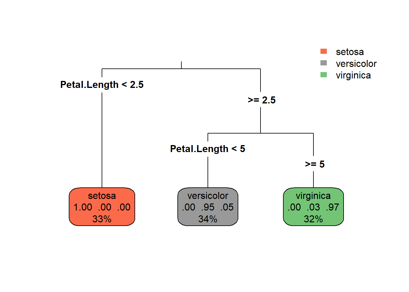
# Use the iris dataset and create a reproducible train/test split
data(iris)
train_idx <- createDataPartition(iris$Species, p = 0.75, list = FALSE)
train <- iris[train_idx, ]
test  <- iris[-train_idx, ]

# Fit a simple rpart tree
fit_rpart <- rpart(Species ~ ., data = train, method = "class", control = rpart.control(cp = 0.01))

# Visualize the tree
rpart.plot(fit_rpart, type = 3, extra = 104, fallen.leaves = TRUE)

# Predict and evaluate
pred_class <- predict(fit_rpart, test, type = "class")
cm <- confusionMatrix(pred_class, test$Species)
cm

Confusion Matrix and Statistics

            Reference
Prediction   setosa versicolor virginica
  setosa         12          0         0
  versicolor      0         11         4
  virginica       0          1         8

Overall Statistics
                                         
               Accuracy : 0.8611         
                 95% CI : (0.705, 0.9533)
    No Information Rate : 0.3333         
    P-Value [Acc > NIR] : 8.705e-11      
                                         
                  Kappa : 0.7917         
                                         
 Mcnemar's Test P-Value : NA             

Statistics by Class:

                     Class: setosa Class: versicolor Class: virginica
Sensitivity                 1.0000            0.9167           0.6667
Specificity                 1.0000            0.8333           0.9583
Pos Pred Value              1.0000            0.7333           0.8889
Neg Pred Value              1.0000            0.9524           0.8519
Prevalence                  0.3333            0.3333           0.3333
Detection Rate              0.3333            0.3056           0.2222
Detection Prevalence        0.3333            0.4167           0.2500
Balanced Accuracy           1.0000            0.8750           0.8125

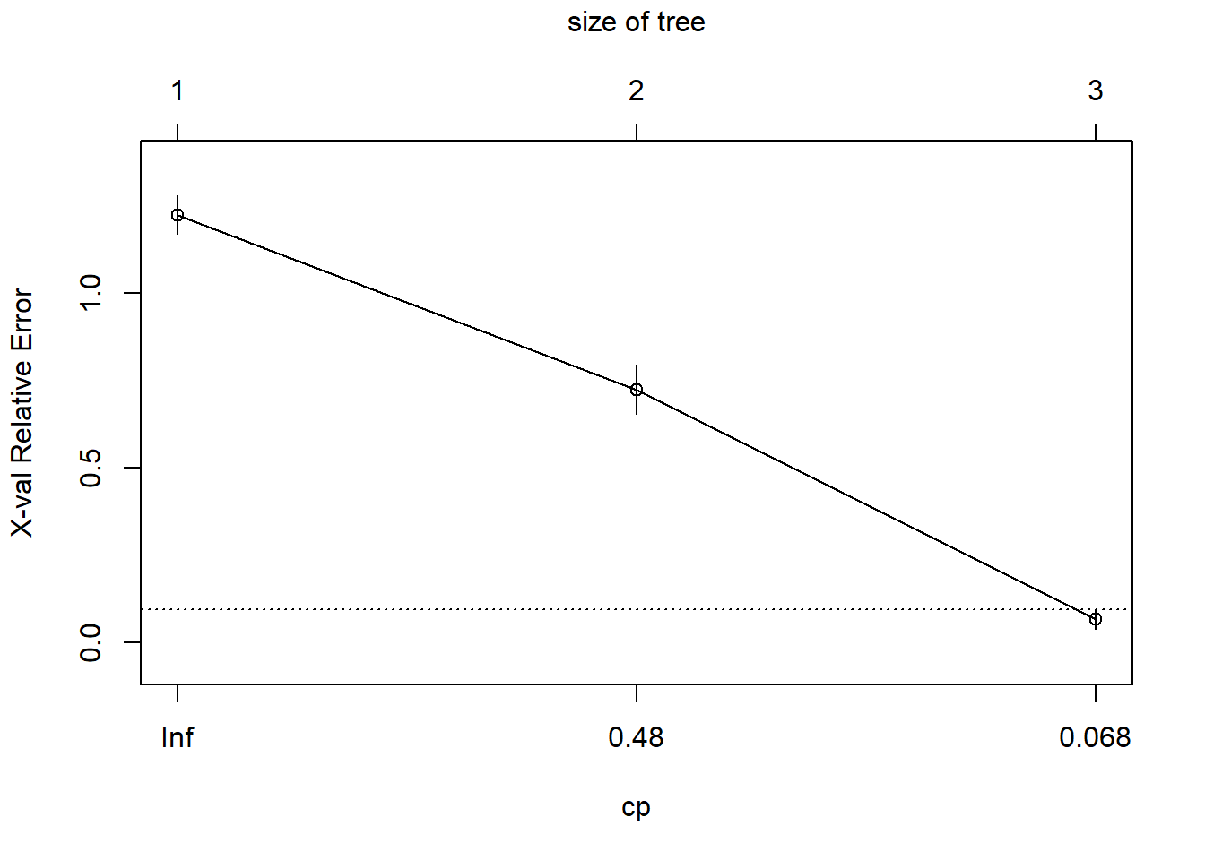
Teaching notes: explain cp (complexity parameter), minsplit, maxdepth, and how pruning works. Use printcp(fit_rpart) and plotcp(fit_rpart) to choose cp.

printcp(fit_rpart)


Classification tree:
rpart(formula = Species ~ ., data = train, method = "class", 
    control = rpart.control(cp = 0.01))

Variables actually used in tree construction:
[1] Petal.Length

Root node error: 76/114 = 0.66667

n= 114 

       CP nsplit rel error   xerror     xstd
1 0.50000      0  1.000000 1.223684 0.054461
2 0.46053      1  0.500000 0.723684 0.070201
3 0.01000      2  0.039474 0.065789 0.028769

plotcp(fit_rpart)

# prune to the cp with lowest xerror or the 1-SE rule
opt_cp <- fit_rpart$cptable[which.min(fit_rpart$cptable[,"xerror"]), "CP"]
fit_pruned <- prune(fit_rpart, cp = opt_cp)
rpart.plot(fit_pruned, type = 3, extra = 104)

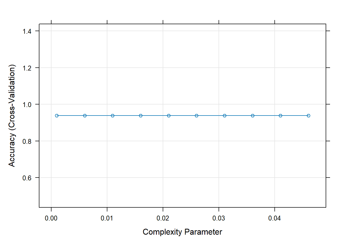
3.5 4. Cross-validation and tuning with caret

ctrl <- trainControl(method = "cv", number = 5, classProbs = TRUE, summaryFunction = multiClassSummary)
set.seed(42)
tune_grid <- expand.grid(cp = seq(0.001, 0.05, by = 0.005))
caret_rpart <- train(Species ~ ., data = train, method = "rpart", trControl = ctrl, tuneGrid = tune_grid)
caret_rpart

CART 

114 samples
  4 predictor
  3 classes: 'setosa', 'versicolor', 'virginica' 

No pre-processing
Resampling: Cross-Validated (5 fold) 
Summary of sample sizes: 92, 93, 90, 91, 90 
Resampling results across tuning parameters:

  cp     logLoss   AUC        prAUC       Accuracy   Kappa      Mean_F1  
  0.001  1.031016  0.9625794  0.04513889  0.9378411  0.9066523  0.9351836
  0.006  1.031016  0.9625794  0.04513889  0.9378411  0.9066523  0.9351836
  0.011  1.031016  0.9625794  0.04513889  0.9378411  0.9066523  0.9351836
  0.016  1.031016  0.9625794  0.04513889  0.9378411  0.9066523  0.9351836
  0.021  1.031016  0.9625794  0.04513889  0.9378411  0.9066523  0.9351836
  0.026  1.031016  0.9625794  0.04513889  0.9378411  0.9066523  0.9351836
  0.031  1.031016  0.9625794  0.04513889  0.9378411  0.9066523  0.9351836
  0.036  1.031016  0.9625794  0.04513889  0.9378411  0.9066523  0.9351836
  0.041  1.031016  0.9625794  0.04513889  0.9378411  0.9066523  0.9351836
  0.046  1.031016  0.9625794  0.04513889  0.9378411  0.9066523  0.9351836
  Mean_Sensitivity  Mean_Specificity  Mean_Pos_Pred_Value  Mean_Neg_Pred_Value
  0.9369048         0.969127          0.9509259            0.9728704          
  0.9369048         0.969127          0.9509259            0.9728704          
  0.9369048         0.969127          0.9509259            0.9728704          
  0.9369048         0.969127          0.9509259            0.9728704          
  0.9369048         0.969127          0.9509259            0.9728704          
  0.9369048         0.969127          0.9509259            0.9728704          
  0.9369048         0.969127          0.9509259            0.9728704          
  0.9369048         0.969127          0.9509259            0.9728704          
  0.9369048         0.969127          0.9509259            0.9728704          
  0.9369048         0.969127          0.9509259            0.9728704          
  Mean_Precision  Mean_Recall  Mean_Detection_Rate  Mean_Balanced_Accuracy
  0.9509259       0.9369048    0.3126137            0.9530159             
  0.9509259       0.9369048    0.3126137            0.9530159             
  0.9509259       0.9369048    0.3126137            0.9530159             
  0.9509259       0.9369048    0.3126137            0.9530159             
  0.9509259       0.9369048    0.3126137            0.9530159             
  0.9509259       0.9369048    0.3126137            0.9530159             
  0.9509259       0.9369048    0.3126137            0.9530159             
  0.9509259       0.9369048    0.3126137            0.9530159             
  0.9509259       0.9369048    0.3126137            0.9530159             
  0.9509259       0.9369048    0.3126137            0.9530159             

Accuracy was used to select the optimal model using the largest value.
The final value used for the model was cp = 0.046.

plot(caret_rpart)

# evaluate on test
pred_caret <- predict(caret_rpart, test)
confusionMatrix(pred_caret, test$Species)

Confusion Matrix and Statistics

            Reference
Prediction   setosa versicolor virginica
  setosa         12          0         0
  versicolor      0         11         4
  virginica       0          1         8

Overall Statistics
                                         
               Accuracy : 0.8611         
                 95% CI : (0.705, 0.9533)
    No Information Rate : 0.3333         
    P-Value [Acc > NIR] : 8.705e-11      
                                         
                  Kappa : 0.7917         
                                         
 Mcnemar's Test P-Value : NA             

Statistics by Class:

                     Class: setosa Class: versicolor Class: virginica
Sensitivity                 1.0000            0.9167           0.6667
Specificity                 1.0000            0.8333           0.9583
Pos Pred Value              1.0000            0.7333           0.8889
Neg Pred Value              1.0000            0.9524           0.8519
Prevalence                  0.3333            0.3333           0.3333
Detection Rate              0.3333            0.3056           0.2222
Detection Prevalence        0.3333            0.4167           0.2500
Balanced Accuracy           1.0000            0.8750           0.8125

Notes: caret::train automates CV and tuning. Explain multiClassSummary (accuracy, Kappa, etc.).

3.6 5. Feature importance & interpretation

# Variable importance from rpart:
varImp(fit_rpart)

              Overall
Petal.Length 70.25918
Petal.Width  70.25918
Sepal.Length 35.26587
Sepal.Width  20.46939

# For caret model:
varImp(caret_rpart)

rpart variable importance

             Overall
Petal.Width   100.00
Petal.Length  100.00
Sepal.Length   29.72
Sepal.Width     0.00

Discuss how importance is computed (split improvement) and limitations.

3.7 6. Partial Dependence Plots (PDPs)

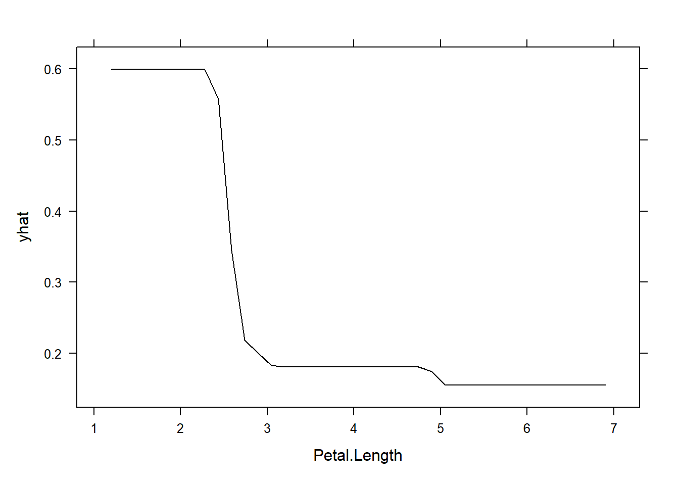
Goal: show marginal effect of a feature on predicted probability (or prediction) while averaging out other features.

3.7.1 6.1 PDP with `pdp`

# Use the caret-trained model (wrap predict function if necessary)
# pdp works with models that have a predict method returning probabilities. We'll use the randomForest wrapper as an example.
rf <- randomForest(Species ~ ., data = train)

# Partial dependence for Petal.Length vs class setosa (probability)
pdp_pl <- partial(rf, pred.var = "Petal.Length", plot = TRUE, prob = TRUE, which.class = "setosa")
print(pdp_pl)

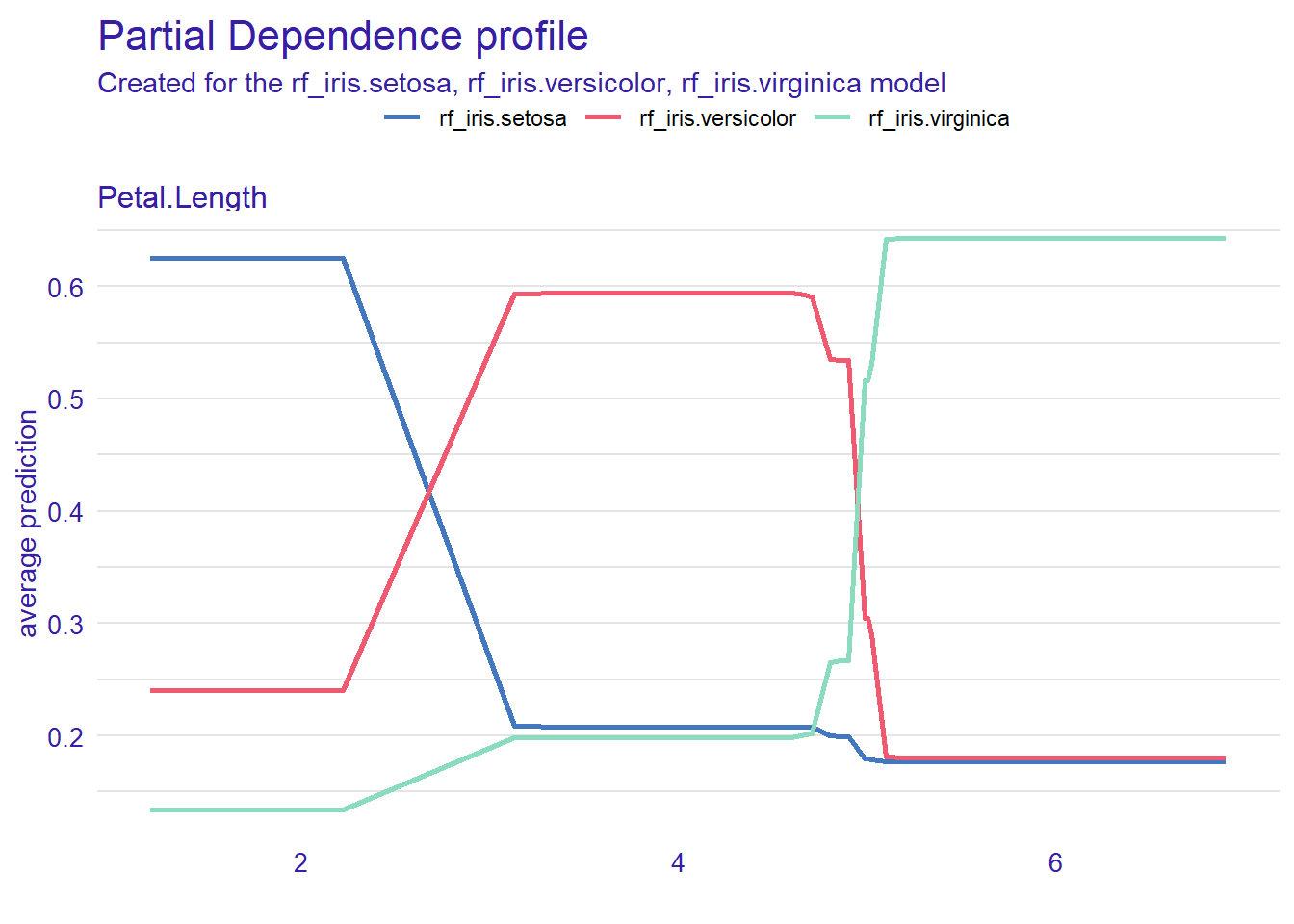
3.7.2 6.2 PDP with `DALEX`

# Create an explainer
explainer_rf <- explain(rf, data = train[,1:4], y = train$Species, label = "rf_iris")

Preparation of a new explainer is initiated
  -> model label       :  rf_iris 
  -> data              :  114  rows  4  cols 
  -> target variable   :  114  values 
  -> predict function  :  yhat.randomForest  will be used (  default  )
  -> predicted values  :  No value for predict function target column. (  default  )
  -> model_info        :  package randomForest , ver. 4.7.1.1 , task multiclass (  default  ) 
  -> predicted values  :  predict function returns multiple columns:  3  (  default  ) 
  -> residual function :  difference between 1 and probability of true class (  default  )
  -> residuals         :  numerical, min =  0 , mean =  0.01891228 , max =  0.34  
  A new explainer has been created!

# Profile (partial dependence) using DALEX
p <- model_profile(explainer_rf, variables = "Petal.Length", N = 50)
plot(p)

Teaching caveats: PDPs show average marginal effects and can be misleading with strong feature interactions. Use two-way PDPs or ICE plots for heterogeneity.

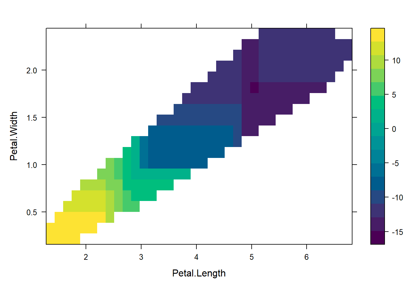
3.8 7. Individual Conditional Expectation (ICE) and 2D PDPs

# ICE using pdp
ice_pl <- partial(rf, pred.var = "Petal.Length", ice = TRUE, plot = TRUE, which.class = "setosa")

# 2D PDP for Petal.Length and Petal.Width
pdp_2d <- partial(rf, pred.var = c("Petal.Length", "Petal.Width"), chull = TRUE)
plotPartial(pdp_2d)

3.9 8. Model comparison: Decision Tree vs Random Forest

# Fit Random Forest and compare
rf_fit <- randomForest(Species ~ ., data = train)
pred_rf <- predict(rf_fit, test)
cm_rf <- confusionMatrix(pred_rf, test$Species)
cm_tab <- rbind(tree = cm$overall[names(cm$overall) == "Accuracy"], rf = cm_rf$overall[names(cm_rf$overall) == "Accuracy"])
cm_tab

      Accuracy
tree 0.8611111
rf   0.9444444

Discuss trade-offs: interpretability (tree) vs performance (RF), stability, and overfitting.

3.10 9. Automated tests for classroom (sanity checks)

# 1) Ensure tree predictions have reasonable accuracy (> 0.7 on iris test)
acc_tree <- cm$overall["Accuracy"]
stopifnot(acc_tree >= 0.7)

# 2) PDP returns a data.frame and includes Petal.Length values
pdp_res <- partial(rf, pred.var = "Petal.Length", prob = TRUE, which.class = "setosa", plot = FALSE)
stopifnot(is.data.frame(pdp_res))
stopifnot("Petal.Length" %in% names(pdp_res))

list(tests = "all passed", tree_accuracy = acc_tree)

$tests
[1] "all passed"

$tree_accuracy
 Accuracy 
0.8611111

3.11 10. Exercises and in-class tasks

Exercise A: Build and prune a decision tree on the wine or iris dataset; show how pruning affects depth and accuracy.

Exercise B: Compute PDPs for two top features in a caret-tuned model and interpret whether they are monotonic or have thresholds.

Exercise C (advanced): Use iml to compute Shapley values for a small set of observations and compare with PDP insights.

End of Module 2 — Decision Tree Analysis & Partial Dependence